THE NERC MST RADAR FACILITY AT ABERYSTWYTH
Doppler spectra files
Owing to the relatively limited data storage capacity available when the MST radar was built in 1989, the Doppler spectra files were designed with volume minimisation in mind. Power spectral density values were pre-compressed so that they could be stored within just 8 bits. However, the format of these files is non-standard and some effort is required to implement appropriate decompression routines. Doppler spectra from the new acquisition system are stored in standard netCDF files making them much easier to access.
Availability of different versions of MST Radar data products
Version-0 (v0) and version-2 (v2) signal processing programs were both designed specifically to operate on the old-style Doppler spectral files. Since version-3 (v3) processing (which was introduced in January 2006) has been demonstrated to be superior to both v0 and v2 processing, it was the only one modified to operate on Doppler spectral files produced by the new acquisition system. Consequently no v0 or v2 data products are available for dates after 6th February 2007.
Changes in signal and noise powers for observations made after 6th February 2007
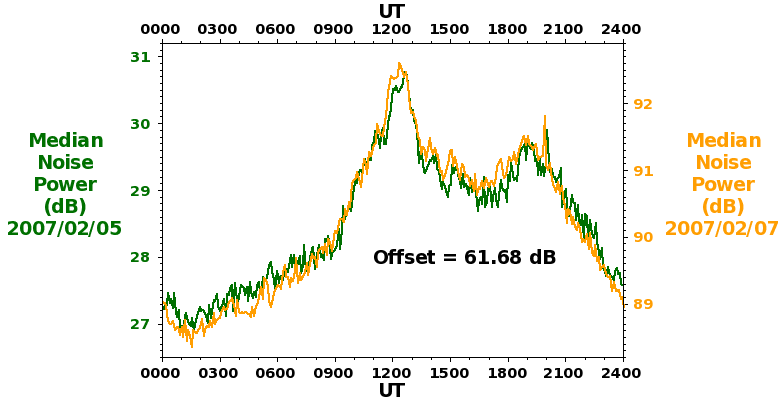
There is a step change of +61.7 dB in signal and noise powers for observations made after 6th February 2007. This is because the power spectral densities are no longer being re-scaled in order to aid data volume compression (as mentioned above). Noise and signal levels are affected equally. The plot below shows the diurnal variations in the median noise power (over vertical-beam ST-mode profiles) for 5th and 7th February 2007. The time variations are primarily a result of changes in the (46.5 MHz) cosmic noise, which explains the extremely high degree of correlation between the two curves. The same pattern of variation is repeated at a slightly earlier time each day in a cycle over the course of a year.
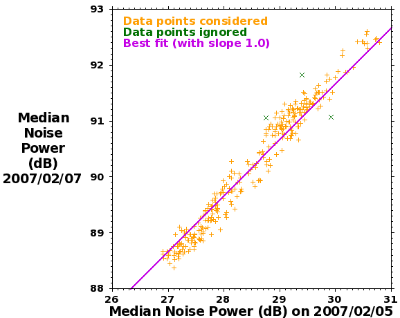
The magnitude of the offset was calculated by regression analysis as shown in the plot below. The best fit line was constrained to have a slope of 1.0, though a free fit results in a value slightly closer to 1.1 (as is evident in the time series curves above).