 THE NERC MST RADAR FACILITY AT ABERYSTWYTH
PSD_linear_units = 10.0^(PSD_dB/10.0)
Positive values of Doppler velocity imply motion away from the radar. The number of velocity bins within a spectrum is given in the spectral and radial data files by by the variable number_of_complex_samples_in_discrete_fourier_transform, abbreviated here as N_DFT. Velocity bin numbers (b) run from (-N_DFT/2) to (N_DFT/2 - 1). The corresponding Doppler velocity values (v_Doppler), which are stored by the spectral file variable doppler_velocity, are given by:
where the spacing between velocity bins (delta_v_Doppler) is stored by the radial file variable spectral_velocity_bin_spacing. Note that spectra are cyclic about the Nyquist velocity, i.e. about velocity bin (-N_DFT/2).
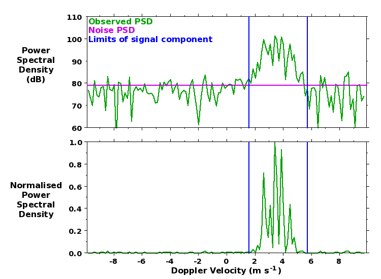
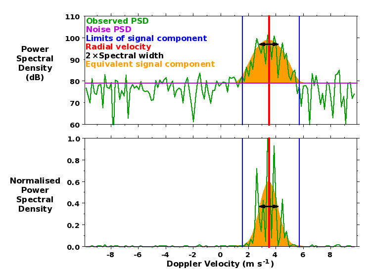
Observed spectra typically consist of a single (quasi-Gaussian) radar return signal component (although there are sometimes additional signal components) superimposed on a background of white noise. The latter implies quasi-constant PSD values at all velocity bins.
Removal of dc contamination
DC biases in the raw radar samples lead to contamination of the PSD for the zero-Doppler-velocity velocity bin, i.e. at b = 0. This must be removed from the recorded spectra before processing can begin. If a Hanning rather than a Rectangular window is used in deriving the spectra (this choice is recorded by the spectral and radial file variable data_weighting_window_index), the contamination is additionally spread to the velocity bins to either side, i.e. it affects velocity bins from (b = -1) to (b = +1). The contamination is typically removed by replacing the PSDs with values linearly interpolated between those at the velocity bins to either side of affected region. The dc contamination has been removed from the spectrum shown above.
Determination of (mean) noise PSD
The (mean) noise PSD (PSD_noise) is determined by the method of Hildebrand and Sekhon (1974). It is shown by the magenta line in the figure above. It can typically only be seen in the log plots as it tends to be very small compared to the peak signal PSD. The noise power in linear units (P_noise_linear_units) is simply the noise PSD integrated across the width of the spectrum:
This is stored in dB units by the radial file variable noise_power (abbreviated here as P_noise_dB). The noise PSD in dB units can therefore be derived from the recorded noise power as:
For spectra derived using a Rectangular window, leakage from strong signal components can affect all velocity bins - see e.g. Hooper (1999). This leads to an overestimate of the noise level, which is otherwise expected to be constant at all range gates. A better estimate of noise level can therefore be obtained by taking the median value over all range gates. The noise power is dominated by broad-band lower-VHF galactic radiation, which undergoes a distinct quasi-diurnal variation of almost 4 dB amplitude.
Determination of signal component velocity bin limits
A smoothed (linear) spectrum is derived by applying a 5-velocity-bin running-mean (cyclically) to the observed PSDs. The velocity bin limits of the signal component are determined by first locating the peak value of the smoothed PSD. The ratio of this value to the mean noise PSD, in dB units, is recorded by the radial file variable peak_smooth_psd_to_noise. Note that this is a measure of detectability and is not the same as the signal-to-noise ratio, which is typically defined as the ratio of the signal power to the noise power. The smoothed PSD envelope is followed out to either side of this peak location until:
- the value drops below the noise PSD
- the value drops below 0.01 of the peak smoothed PSD value, if
this is reached before dropping below the noise PSD. This condition
is particularly important where use of a Rectangular window has led
to spectral leakage. It prevents low PSD values at the edges of signal
components from having a disproportionately large effect on the
spectral width values. Such low values would have a negligible
contribution to the total signal power power - see e.g. Hooper (1999).
- it encounters a local minimum for which the smoothed PSD value is less than 0.1 of the peak smoothed PSD value. This condition is important for resolving partially-overlapping clear-air (i.e. desirable) and unwanted signal components.
These (inclusive) limits - recorded by the radial file variables first_velocity_bin_number and final_velocity_bin_number, but abbreviated here as b1 and b2 - are shown by the blue lines in the figure above. During the process of signal identification, the observed spectrum is first extended with a copy of itself being wrapped around the Nyquist velocity bin to either side, i.e. (b = -N_DFT/2) and (b = +N_DFT/2). A partially velocity-aliased signal component, i.e. one which is apparent at both Doppler velocity bin extremes of the original spectrum, is indicated in the radial files by having ones of its velocity bin limits being extended beyond the expected range of (-N_DFT/2) to (N_DFT/2 - 1).
Calculation of the principal parameters for the signal component
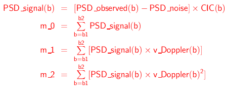
The three lowest-order moments (m_0, m_1, and m_2) of the signal component are calculated from the the PSDs (in linear units) within the velocity bin limits which have been:
- Corrected for noise, i.e. by subtracting the mean noise PSD
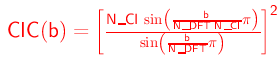
- Compensated for the low-pass filtering effect of coherent integration by multiplying them by a factor CIC - see. e.g. Rastogi (1983). This has a value of 1.0 at (b = 0) and of up to a few dB at the edges of the spectrum.:
Following Woodman and Guillen (1974) or Woodman (1985):
The signal component power (P_signal), radial velocity (v_R) and spectral width (σ_w) are given by:
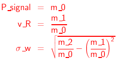
They are stored by the radial file variables signal_power, radial_velocity, and spectral_width, respectively. These can be used to define the magnitude, the central location and the standard deviation, respectively, of an equivalent Gaussian signal component - shown by the orange feature in the figure below - which give rise to the same values of the three lowest-order moments.
- References:
- P. H. Hildebrand and R. S. Sekhon, Objective
determination of the noise level in Doppler spectra Hildebrand,
J. Applied. Met., 13, 808-811, 1974
- D. A. Hooper, Signal and noise level estimation for narrow spectral width returns observed by the Indian MST radar, Radio Sci., 34, 859-870, 1999
- P. K. Rastogi, A note on the use of coherent integration in periodogram analysis of MST radar signals, Handbook for MAP, 9, edited by B. Edwards, Sci. Comm. on Sol.-Terr. Phys. Secr., Boulder, Colorado, pp 509-512, 1983.
- R. F. Woodman, Spectral moment estimation in MST radars, Radio Sci., 20, 1185-1195, 1985
- R. F. Woodman and A. Guillen, Radar observations of winds and turbulence in the stratosphere and mesosphere, J. Atmos. Sci., 31, 493-505, 1974
- D. A. Hooper, Signal and noise level estimation for narrow spectral width returns observed by the Indian MST radar, Radio Sci., 34, 859-870, 1999